The goal of this project was to turn a full GJR-GARCH volatility model into a compact neural surrogate that reproduces its return distributions with high-level accuracy. This required more than training a network. We first reduced the model to its essential shape, simulated a quadrillion simulation steps at high fidelity, distilled the results into stable distributional targets, and trained lightweight mixture-density networks that deliver accurate forward densities in real time.
This article explains the main ideas behind that process: how the model is normalized, how the dataset is constructed, why we learn cumulative distributions, and how Gaussian mixtures make pricing both fast and consistent.
Understanding and Reducing the Model to Its Essential Shape
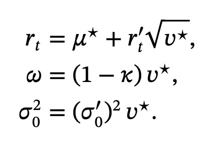
Volatility models contain symmetries that do not affect the shape of returns. Adding a constant shifts the mean, and multiplying by a positive number rescales variance. Different parameter sets can therefore generate identical return behaviour. Before generating data, we map every configuration to a Dimensionless Reduced Form (DRF) where the long-run variance is fixed to one, the drift is zero, and time is measured in units of the mean reversion scale. Only the parameters that shape volatility dynamics remain.
This reduction ensures each training point represents a truly distinct model behaviour and prevents the neural network from learning redundant patterns. It also keeps the simulation domain economically valid by enforcing variance positivity and persistence below one. With the model in DRF coordinates, simulation and learning become more stable, and the resulting surrogate behaves consistently across the entire parameter space.
Why We Learn CDFs Instead of Paths or Histograms
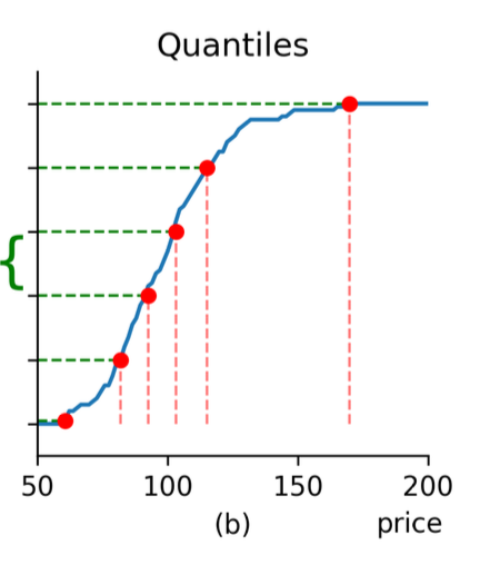
To learn a full return distribution, we need a representation that is smooth, stable, and meaningful for pricing. The cumulative distribution function (CDF) is ideal: it captures all distributional information, handles the tails naturally, and avoids the arbitrary choices required by histograms or kernel fits. Because it is monotone and well behaved across the entire domain, a CDF is straightforward for a neural network to approximate.
Our loss compares the predicted and Monte Carlo CDFs at fixed quantile levels. This choice is directly aligned with the goal of pricing accuracy. For lognormal mixture models, the CDF deviation determines the error in option values across strikes, so reducing the CDF loss reduces pricing error in a predictable way. The result is a target that reflects the true structure of the distribution and allows the surrogate to focus on the shape of uncertainty rather than noise from Monte Carlo paths.
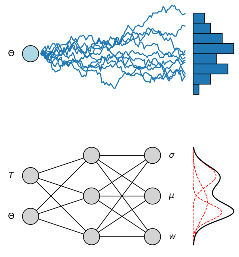
A Quadrillion Simulation Steps Reduced to a Small Neural Model

Each parameter configuration is simulated with 10 million Monte Carlo paths of a 1,000 time steps, across 128,000 combinations sampled using a Sobol sequence. This results in about one quadrillion time-step updates. Running this workload on a 50-GPU cluster for three days produces clean empirical distributions with very low sampling noise, which is crucial because the surrogate cannot exceed the accuracy of the data it is trained on.
The distilled dataset is compact and published openly at HuggingFace. From this data we train two small networks: a browser-ready 2×32 model with a CDF error around three times ten to the minus four, and a larger 2×128 model with error near one times ten to the minus four. Although small, these networks encode the behaviour of a simulator that normally requires minutes of computation for a single configuration.
GJR-GARCH density dataset on Hugging Face
The full training dataset for this project is available as a public resource. It contains distilled return distributions for 128 000 parameter configurations, generated from roughly one quadrillion simulated time steps in GJR-GARCH.
You can explore the dataset, inspect the schema, and plug it into your own experiments.
View dataset on Hugging FaceUsing Gaussian Mixtures for Fast and Consistent Pricing
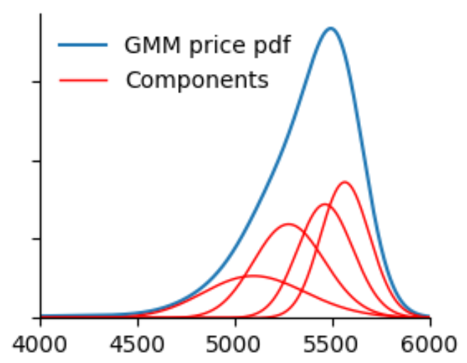
The surrogate predicts the return distribution as a Gaussian mixture. This choice is practical and mathematically convenient. Mixtures can approximate a broad class of shapes, including skewed and heavy-tailed distributions. They also have a simple interpretation in option pricing: each Gaussian component produces a lognormal distribution for the forward, and every option value becomes a weighted sum of Black-formula prices.
A small adjustment guarantees that the mixture reproduces the correct forward price exactly. This maintains risk-neutral consistency without adding complexity. Once the mixture is known, all strikes and maturities follow from closed-form formulas, so the model delivers full volatility surfaces and prices with negligible latency.
Covering the Entire Parameter Space Reliably
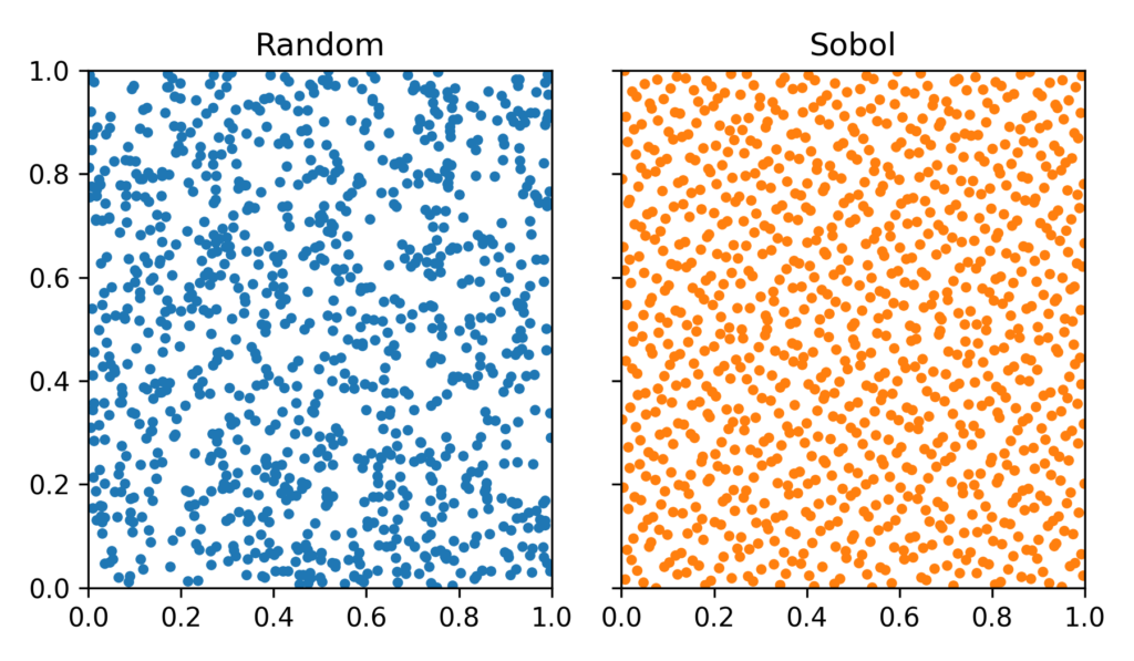
A surrogate model is only trustworthy if it has seen all relevant behaviours of the underlying process during training. Uniform random sampling leaves gaps, which is problematic for high-dimensional parameter spaces. Instead, we use Sobol low-discrepancy sequences to explore the admissible parameter domain evenly, including boundary regions where volatility is persistent or responds strongly to negative shocks.
In combination with the DRF transformation, this guarantees that the network learns by interpolation inside a well-covered domain rather than extrapolation beyond it. The surrogate therefore behaves predictably and smoothly across the entire parameter space, including scenarios that are rare but important for stress testing or risk analysis.